Gabor Wavelets

Similar to the system of Lades et al. [5], we apply a wavelet transform based on the Gabor kernel

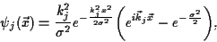$$\psi_{j}(\vec{x}) = \frac{k_{j}^{2}}{\sigma^{2}} e^{-\frac{k_... ...iggl(e^{i\vec{k}_{j}\vec{x}}-e^{-\frac{\sigma^{2}}{2}}\biggr),$$ (1)

where

$$\vec{k}_{j}=\binom{k_{\nu}\cos\phi_{\mu}}{k_{\nu}\sin\phi_{\m... ...{-\frac{\nu+2}{2}}\pi,\thickspace \phi_{\mu}=\mu\frac{\pi}{8}.$$ (2)

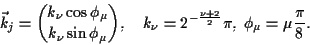
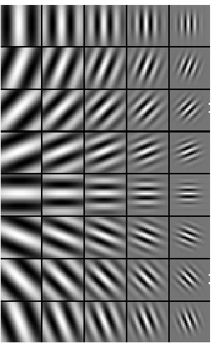
All the Gabor wavelets are created from this kernel by dilation and rotation. The 40 wavelets created from indices $\nu\in\{0,...,4\}$ (size) and $\mu\in\{0,...,7\}$ (orientation) are shown in figure 4. These wavelets are convolved with the image, and we keep the value of the center pixel. This provides us with a feature vector of 80 complex coefficients, but we only keep the amplitudes for classification.

  

Figure 4: The Gabor wavelets.